May 2022 (Original ≽)
Maintenance »
Question: Is the information maintained over time?

Answer: Yes, because if it were not so, physical experiments would not be valid evidence of something that happened. The information from the observed process would be unreliable if it were not able to reach the operator exactly as it was formed there.
It is similar with talking, sending messages by phone, via radio, TV, or third-party media. The internet would be impossible if information could not be transmitted in space and time. At the same time, it, like the impulse of the billiard ball, can be directed and maintained to the place of delivery. Then the change of momentum (p) on the path (x) will change it, because the information is equivalent to the action (px).
Information is the equivalent of both the product (Et) of energy (E) and time (t), which is another expression for physical action. Therefore, the total energy of a given physical system will be equal in equal time intervals, because the law of conservation of information applies. Hence, the higher the observed energy, the slower the relative time of the system.
This observation, by the way, reveals the property of inertia of information, which is not the topic of the current answer. By slowing down the information becomes lazy, a greater force is needed to start it, a greater impulse to overcome it, from which we infer that energy and momentum in that situation are proportional. The inertia of information is also a matter of principled minimalism, both its changes and emissions.
By dilating relativistic time due to the uniform inertial motion of the system, observing the same information in the part of the duration of one's own (proper) observer results in relatively higher energy as many times as that time interval is less than one's own, because the product of energy and duration is actually constant. The same happens with the relativistic contraction of the path and the increase of the momentum.
Due to the constant speed of light in vacuum (c ≈ 300 000 km/s), along the direction of movement of a given system, the relatively observed traversed paths, for the speed of light, will be constant in the corresponding parts of their proper (own) time. Therefore, the relative contraction of lengths is accompanied by the corresponding dilatation of time, known to us from the theory of relativity (Einstein, 1905), from which the constancy of the pseudo surface (tx) derives.
There is no information without time and place, it is two-dimensional, so the same constancy does not apply to, say, real surfaces (like xy). But these are just hints, less than the "tip of the iceberg" of what I have to tell you about the law of conservation of information.
Channel »
Question: What about possible errors in the transmission of information?
Answer: Uncertainty in principle also implies errors in communication. In the case of a natural number n ∈ ℕ of the sender and receiver of the signal, this will mean that there are some probabilities kij ∈ (0,1) of receiving the i-th and sending the j-th signal. When ∑i kij = 1 is valid for sending the j-th, then the arrival of that signal in the form of one of the given (i-th) makes the probability distribution. Also, if the sum of all j is one, ∑j kij = 1, for a fixed received i-th, then sending that received form the probability distribution.
This is how the transmission channel is defined, the matrix K = (kij) whose coefficients are conditional probabilities. If the sequence or vector is the probability of the signal at the input p = (p1, ..., pn), the output of the channel will be q = (q1, ..., qn), where by matrix multiplication we get q = Kp. Let us now consider the introduction and conservation law of information into this equation.
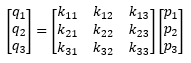
In the picture on the right we see an example of this matrix equation, for channel 3 × 3. The probabilities on the diagonal of the transmission matrix (kii) must be different from the others of their row (column) in order to have a chance of identifying the sender based on the receiver. Namely, if all these probabilities were equal to each other, only noise would come out of the transmission channel. But nature does not like equality (Equality).
The message sent to the recipient would be all the clearer because the out-of-diagonal probabilities (kij, for i ≠ j) of the matrix are smaller. It is not necessary for them to be zeros, for example, for the transmission of the j-th message to be error-free, but only for the diagonal probability to be greater than the sum of the others in that row (column). If there is such a situation in each row, that each diagonal element of the matrix is larger than the sum of the others, then there is a transfer. Reconstruction of the sent is possible from the received.
Theorem. Condition |kii| > ∑j:j≠i |kij| (i, j = 1, 2, ..., n) is enough for K ≠ 0.
Proof: Suppose the opposite, that det K = 0. Then the system of linear homogeneous equations ∑j kijpj, has a nontrivial solution, where ∑j |pj| > 0. Let |pi| = max{pj} and in the homogeneous system we notice the equation
If in the proof we take the minimum |pi| instead of the maximum and consistently, we will prove: when each diagonal element of a given matrix is less than the sum of the others of its row, then the determinant of the matrix is different from zero. Note that this is true for all square matrices of type n × n and that the coefficients kij do not have to be real numbers either (Information).
When we work with classical information and probabilities expressed by real numbers from 0 to 1, then the condition of the inequality theorem is kii > ½ for every i = 1, 2, ..., n, the same if all kii < ½. The determinant of the matrix is then different from zero, the corresponding system of linear equations will be regular, invertible, which means that the originals (p = K-1q) can be calculated on the basis of copies (p = K-1q).
The invertibility of the system of equations, i.e. the regularity of the corresponding matrix (det K ≠ 0) means the memory of the characters based on the images, and that there is a maintenance of the information transmitted by the channel. The attitude that the law of conservation information applies in nature, according to the previous, implies that nature does not tolerate equality (Levelness).
In short, when all the chances of transmitting the i-th signal in the i-th order are greater than 50 percent, then the information remains preserved. In the extreme second case, when they (kii) are less than 50 percent, we have the same, but decoding is more difficult, because the information is then present, but suppressed, disguised as in the case of lies (The Truth). Answering the question, I was asked, we can say that there are no errors in the transmission of information.
Recursion II »
Question: Are transmission errors increasing through the Channel?
Answer: That's right, it's logical, and it's easy to check with the channel matrix you mention. Let's say it is a matrix K of the second order (2 × 2) with two diagonal elements a ∈ (0,1) and non-diagonal b = 1 - a, whose amounts are the probabilities of transmission. But there is one interesting thing.
By squaring it (K2) we get a matrix of the second order with elements on the diagonal a2 + b2 and outside it 2ab. The sum of both the same rows (or columns) is the square of the binomial (a + b)2 = 1, because a + b = 1, so it is also a transmission channel (a pair of signals in a pair of signals). It is a connected transmission of information through two consecutive channels K. By induction we can easily prove that the transmission through n = 1, 2, 3, ... such channels is each time a transmission channel (two signals), with a exponential matrix (Kn), diagonal elements an and other bn, and always an + bn = 1.
For example, when a = 0.70 then a2 = 0.58 when a3 = 0.53 thereupon a4 = 0.51 and a5 = 0.50 approximately, after which the first two decimal places are repeated (followed by not all zeros). When a of the basic channel is a larger number (less than one), then a longer composition, a higher degree n, is needed, so that the first one decreases to 0.50. Conversely, with a smaller initial a (down to ½) this string will be shorter.
However, when a < ½ more interesting situations arise. The sequence a, a2, a3, ... of the elements of the diagonal of the exponential matrices (Kn) becomes alternate, from below 0.5 and above. For example, starting by a = 0.3 it will be a2 = 0.58 then a3 = 0.47 when a4 = 0.51 and a5 = 0.49 to continue constantly oscillating around 0.50. The informatic explanation is as follows.
When in the basic matrix of channels, we have the advantage of transmitting the i-th to the i-th signal, probability a > 1/2, by the composition of more such channels, this probability decreases, but still remains favorable (always an > 1/2). The output contains an initial message, but it is increasingly difficult to decode it because it is suppressed, masked, concealed. It is more and more impersonal, with information that is there, but it is reluctant to be emitted. Let's compare this with entropy, which, according to (my) information theory, similarly loses information. In both cases, there is the principle of communication stinginess.
When in the basic matrix of channels (K) we have the disadvantage of transmitting the i-th to the same signal, probability a < 1/2, through connected such channels the message flow oscillates. Its transmission is more certain, then more uncertain, as if "truth" attracts "lies" and this one is again defeated by "truth" (The Truth). This way of vibrating is actually a common occurrence of physical reality, although it is unnoticed until the theory of information (compare with Oscillation).
Determinant |K| = |a2 - b2| = |(a - b)(a + b)| = |(a - b)| < 1, for ab ≠ 0. Namely, both of these numbers are probabilities a, b ∈ (0,1), where a + b = 1. Hence, such mapping compositions are constantly damped (oscillations for |a| < |b|). For n → ∞ it will be |K|n → 0, but for every finite n it |K|n ≠ 0 holds – which is why the composition of the channel keep information.
The point in both cases is the law of information conservation and it is of a principled, universal nature. To my second question (Where did this law of conservation come from?), the better answer is coincidence, I suppose, than that it should be produced from some simple few postulates of the theory itself. Namely, if we assume that the universe does not have such a law, then we would not exist either.
Spin Matrices »
Question: Are there undamped mappings?
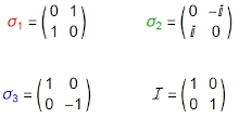
Answer: Yes, there are attenuated data transfer. What's more, quantum mechanics mostly works with such. The picture on the left show’s examples of their "channels". These are Pauli matrices, the solutions of the matrix equation σ2 = I, where the indices 1, 2 and 3 can be replaced by x, y and z, respectively.
It is easy to see that the determinant of each of them is |σ| = 1, including the unit matrix (|I| = 1), so in the style of the previous (Recursion II) we can say that they are "channels without attenuation" and, of course, they store the given information.
In mathematical terms, isometries are those mappings that will form channels without attenuation. All of these are some rotations, and examples in physics are vibrations. I'm talking about just the ones I mentioned recently.
Quantum matrices map vectors of "generalized probabilities" (as opposed to "ordinary" in Channel), with complex coefficients whose squares of modules are the probabilities of finding a particle-wave in certain physically measurable states.
Question: What is a "spin"?
Answer: Spin (rotation, marked with the letter s) is one of the basic properties of elementary particles. We interpret it as an internal moment of impulse. For spin, as for ordinary momentum (product of mass and velocity) and energy, and now for information, the law of conservation applies. It reacts to the magnetic field and affects the movement of electrons. Spin is exclusively a quantum property of particles without their "mate" in classical mechanics.
Like the north-south poles of a magnet, it is made up of pairs of values that can be reduced to opposite half-integers in the case of fermions, or integers for bosons. The quantum operator associated with spin-½ is Ŝk = ħσk/2. The index k denotes an arbitrary Pauli matrix, in the figure above left.
Qubit »
Question: Is there always a lot of zeros in the matrix of undamped mappings?
Answer: Not. The Hadamard matrix H (Quantum Mechanics, 1.1.3 Qubit) has 1 and -1 on the main diagonal, and 1 and 1 on the secondary diagonal, divided all by the root number two (√2) so that its determinant is one. The figure shows its effect on unit vectors: Hex = (ex + ey)/√2 and Hey = (ex - ey)/√2.
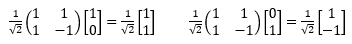
It stores information, moreover, it does not suppress it (its determinant is one), and it does not have a single zero coefficient. It is inverse to itself (H2 = I), so its composition can be represented as an oscillation here and there of a given signal.
Question: What is "qubit"?
Answer: Qubit is a quantum bit. In quantum computing, its counterpart is the binary digit or the bit of the classical computing. Just as a bit is the basic unit of information in a classical computer, a qubit is a basic unit of information in a quantum computer. However, unlike bits, qubits are vector quantities. It contains both possibilities of a given two-way, so-called binary distributions.
Hadamard's matrix of the second order, mentioned, is an example of the transfer of qubits, i.e. two-component vector, the quantum state. Such are the binary distributions of probabilities, the dual random outcomes we see when throwing (unfair) coins. But, unlike gates (switches) of classical electrical circuits (computers), which pass only one of the possible signals, only one component of the distribution vector, in quantum way, the corresponding "gates" pass entire vectors. (Quantum calculus).
Eigenvalues »
Question: What are the characteristic values of the matrix?
Answer: Let M be a square matrix. The roots of the equation det(M − λI) = 0 are called characteristic values of M. Therefore, the numbers λ are characteristic values of M if and only if there is a nonzero vector x such that Mx = λx. Each vector x that will solve the matrix equation Mx = λx is called the characteristic vector associated with the characteristic value λ.
In quantum mechanics, the characteristic value is called "eigenvalue" and the characteristic vector "eigenvector". These names are increasingly used in algebra, because quantum mechanics is its representation.
The number is the (square) "matrix" of the first order (n = 1), and then the corresponding "vector". The linear function f(x) = kx equivalent to such a matrix will have any number x as a characteristic vector associated also with an arbitrary characteristic value of k. Geometrically, it is a function of homothety (stretching or shrinking to the path), or similarity (proportional increase-decrease of the distances of a given figure), i.e. proportionality.
Simply said, the simple linear function f(x) = kx is a measurement. The one-component vector x is the length, or time, kilogram and in general some observables (physically measurable quantity), and k is its quantity. It extended to n = 1, 2, 3, ... component vectors (n-tuple arrays) will be a linear operator, or its corresponding matrix.
Quantum mechanics works with just such, where real numbers are often generated by complex ones. Thus, the above Mx = λx becomes a "homothety", when only real numbers λ are interpreted as real observable. At such a level of physical quantities, we hold observable the possibilities, or distributions of probabilities, of eventual measurement of a given physical quantity within the given circumstances.
It is useful to go to the very bottom of physics, to its current microworld, to notice uncertainties and introduce or understand "information theory" in physics (in my way) and to recognize "information of perception" in the quantum mechanics itself.
Question: Do you have any examples?
Answer: Well, simple linear functions are simple examples. When we say "measured length is 17 meters", we are talking about such a linear function whose characteristic vector is the dimension of length in meters, with its characteristic value of 17.
Another example is unit matrices of arbitrary order (number of n rows / columns). They map vectors (of the order of the matrix) into the same vectors, because they have ones on the diagonal, and all other elements are zero. Therefore, every vector x (of the order of the matrix) with the number λ = 1 will be "characteristic" for the unit matrix, because Ix = 1⋅x.
The third example is the Pauli matrices (Spin Matrices). Each of them will have characteristic values +1 or −1 and characteristic vectors that correspond to them, presented in the following figure (i2 = -1).
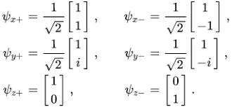
The coefficients of such vectors can be complex numbers (the second pair of these) whose squares of the modules represent the measurement probabilities of a certain observable. The coordinate axes of the observable measure that could appear under given conditions (quantum state), so we see (by simple calculation) that these vectors represent the certainties of the observables.
Question: Why could characteristic values be observable?
Answer: A quantum system is a representation of a vector space (X), whose quantum states are vectors (x ∈ X). States consist of particles of mesons, electrons, hydrogen atoms and the like, and the system is all around that can but does not have to be measured. A linear operator, like M whose matrix is the above-mentioned M, is a quantum process. The set of all vectors of a given characteristic value of any such operator forms a subspace.
Namely, if Mx = λx and My = λy, then the linear combination is:
That is why they make a well-defined space for observers, because measurable physical quantities, physical reality, would mix in a similar way. Secondly, this thesis has already been confirmed with many experiments, without exception. Particles transmit actions, and therefore information, so the same characteristic values become expressions of information theory.
A linear combination of states is again a state with the same observant, its new value, but the same essence. The very notion of "kilograms" will not change by mixing different kilograms of some substances.
Observable »
Question: Do we measure the observable both with the help of characteristic values and with the help of coordinates?
Answer: Yes, that's right. It is this "secret" connection between the eigenvalues of linear operators and the diagonalization of the matrices associated with them.
It can be proved (Channel, Theorem) that inequalities of results when copying create the possibility of recognizing the original. Algebra calls such "invertible" operators, in physics they express "laws of conservation" (momentum, energies, information). If we have an invertible mapping S: x → y, then there is also an inverse S-1: y → x.
We also call invertible operators "regular", because they describe systems of linear equations with regular, unique solutions. We as well call them "similarity", because two operators A and B are "similar" when B = S-1AS is valid. All of the above also applies to the corresponding matrices, because they are equivalent to linear operators, and besides to communications due to equivalence with transmission channels.
Theorem. If B = S-1AS, matrices A and B have the same characteristic values.
Proof: Based on Cauchy-Binet theorem for square matrices, that the determinant of their product is equal to the product of the determinant:
As similar matrices have the same Eigenvalues, they refer to the same subspaces and form one "reality". It follows from the view of (my) information theory that subjects who can communicate (in) directly are (in) directly real. But the opposite is not true, because matrices of the same eigenvalues do not have to be similar, so algebra approves the existences of different such realities.
It is known that we can diagonalize these matrices, and that is the central answer to the question. Diagonal elements give the coordinates of the system, and at the same time the eigenvalues, when both can be reduced to the same observables. In other words, behind the "good" choice of observables (basic physical quantities) and presenting them with coordinates, which we have seen is always possible, the eigenvalues of the process, which are also measurable, will not be "confusingly" different from the starting terms.
Verticality »
Question: Can you explain to me the diagonalization of the matrix?
Answer: Try to understand things like this first. After choosing the observables (basic physical quantities) in a "good" way and representing them with coordinates, which is seen in the above (Observable) as possible, the inherent values of the resulting processes (which are also measurable) will not "confuse" their difference from the original concepts. That is why the diagonalization of the matrix is possible, because of that common denominator.
In other words, the coordinates and eigenvalues are not at odds, if we choose right the first ones. The problem arises by transferring our intuitive ideas of the physics of the macroworld to the microworld, when they are "distorted" as these coordinates. The real cause is a little deeper, in allowing "lies" (mitigating or suppressing the truth) by nature (The Truth), but that is not on the agenda today.
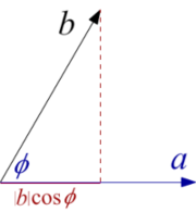
In the picture on the left we see two vectors, two oriented lengths a and b that close the angle φ and the projection of the second on the first, length |b| cos φ. Their scalar product is
By changing the coordinate system, the second record changes, but not the first and third; the intensities of these vectors do not change, neither the angle between, nor the result of scalar multiplication. The coordinate system resembles a scaffold set up to build a building that is eventually removed. Records that we perform during the calculation with coordinates, important in the process of work, and later less important, can be performed in different ways.
Diagonalization of the matrix, i.e. the operator associated with it, is the procedure of calculating new coordinates from the old ones, in order to obtain the best possible ones. Such are mutually perpendicular, because then each of them (by its projection) does not usurp any of the others. Namely, there is no information of perception (vectors) between individual coordinates and the rest of the space, so there is no action between them. The last statement comes from the informatic explanation of routine, the Gram-Schmidt method, orthogonalization (Quantum Mechanics, Orthonormal vectors, 137), which actually does not need interpretation.
Let the vectors a and b, from the image above left, be exactly coordinates. Then an arbitrary vector of that plane is x = αa + βb, so multiplying scalarly follows:
With the orthogonalization of the coordinate system, they coincide with the eigenvalues of the operators, both with possible observables, and the diagonalization of the corresponding matrices occurs.
Unitary spaces »
Question: What are unitary spaces?
Answer: In information theory, "unitary" has a meaning similar to quantum mechanical (Hilbert space) applications of unitary spaces of algebra. In this case, ⟨a, b⟩ = a ⋅ b, where a and b are vectors of a given space, and further as seen in the previous answer (Verticality). Scalar multiplication of vectors is interpreted by "information of perception" between vectors, subjects a and b, their greater adaptation by greater parallelism (a || b), and the verticality of participants (a ⊥ b) by the absence of mutual observation.
It is assumed that the scalar (so-called "inner" or "point") product is conjugately symmetric, ⟨y, x⟩ = ⟨x, y⟩*, so ⟨x, x⟩ = |x|2 is a real number. But it is required that it is always |x| ≥ 0, and zero for the zero-vector only. Additionally, the product is linear by the first argument, ⟨ax + by, z⟩ = a⟨x, z⟩ + b⟨y, z⟩, and then, due to the previous one, it is conjugately linear by the second.
In probability theory, which we partly apply in information theory, instead of "almost everyone" we write shorter "everyone", which is the choice of probability 1. Due to the law of large numbers it could mean "just everyone" in macro-physics, but not in lower particle level of micro-physics. Within the domain of quantum physics, one should count on occasional communications, i.e. interactions of "orthogonal vectors" as well.
Question: Does any conservation law apply here?
Answer: Yes, the law of conservation of information perception has a special meaning here. It can explain the metrics of geometries (flat and curved spaces), and by the way, the intervals of the theory of relativity. In terms of the above answer, the "well" chosen coordinates will become observable of the observed quantum system to which the law of conservation total perception applies. If the multiplied vectors contain the sums of all possible perceptions of the system, then the equality ⟨x, y⟩ = const is possible, which then becomes a kind of law of conservation of information perception.
The square of the modulus (length) of the unit vector u is |u|2 = ⟨u, u⟩ = 1. When we project such on the k-th coordinate of the Cartesian rectangular system (Ox1...xn) the projection is the length of the cosine of the angle, cos φk = cos ∠(u,xk), which vector coincides with that axis. This is known from elementary analytical geometry.
However, the product of two such projections, the first with the projection of the k-th orth (unit vector of the orthogonal coordinate system) on a given vector, will give the square of the mentioned cosine which then represents the probability of interaction between the vector u and xk axes. The sum of the probabilities of interactions of all axes (k = 1, 2, ..., n) is one, when they form a complete set of independent events. This is, in short, the content of the idea of Born probability (Quantum Mechanics, 1.1.6 Born rule).
From the constancy of the cumulative probability of distribution, ∑k cos2φk = 1, follows the mentioned law of conservation the overall perception, after carefully choosing the method of measurement. We transmit this property of quantum mechanics more broadly into applications, through storms that cannot be easily calmed down, all the way to information of perception of living beings (Aging), which due to this law of conservation cannot get rid of excess information too quickly and become some inanimate beings.
Question: Can this "information" be negative numbers?
Answer: The information of perception treated in this way uses not only negative real numbers, but also complex ones. For example, let’s put:
Question: Can this be generalized?
Answer: This is easily generalized to the case when the component vectors x1, ..., xn are composite. Namely, from the system of equations xi = ∑j βijvj, where vj are some elementary vectors, by composition (matrix multiplication) we get the upper system, we express the given vectors (observable) as elementary.
Given the matrix equation (Gα = 0), the set of vectors xj will be linearly dependent only if det G = 0. Namely, when this determinant disappears, the linear system has an excess of equations and some variables (alpha) can be expressed by others. And if the determinant is not zero, then there is only a trivial solution (all alphas are zeros).
Question: Yes, it is a known feature of a system of linear equations. Do you have another way?
Answer: We find the same property of this system by observing volumes. In the space of one vector x, the Gram determinant is the square of the length of the vector (|G| = ⟨x, x⟩ = |x|2). The Gram determinant of the space of two vectors is the square of the area of the rectangles they span:
In general, the Gram determinant is the square of the volume of an n-dimensional square spanned by a system of the same number of orthogonal vectors, so when |G| = 0 will be that at least one of the vectors is not independent, but lies in the space of the others. When the vectors xk form a linearly independent system, this method can further prove that the Gram determinant is a positive number.
The third way is information method. If (Channel) is separated from the content of 3-D essentially different data packed in a container, only one slice is sent and thus saved, all but one 2-D rectangle is lost – it will not be possible to decipher all originals from the copy. More generally, if we extract one n-1-dim "slice" from the n-dim "square" of such data – there is no complete memory in the copy about the original, and the determinant of the matrix is zero (|G| = 0).
Question: Have we gone too far in interpreting vectors?
Answer: Not at all. Working with negative and complex numbers (scalars), the final results do not have to be the same. However, they all have some messages and theoretical consequences, but they are not the topic here. What is the topic is the conclusion that we interpret vectors as quantum states (particles), then as observable, including perceptions that we do not have to have senses from our macro-world, but we also interpret vectors as information.
These are the ranges of application of the algebra of unitary spaces, as far as (my) information theory is concerned.
Minimalism »
Question: Is the principle of minimalism of information seen somewhere in the algebra of operators?
Answer: Yes, that minimalism is visible, but I don't know how much it is really noticed in the application of algebra. I will explain, I hope in simple enough words, although there is hardly anything simple in that topic.
We have seen (Channel) that diversity is a necessary condition for "memory" and the law of conservation information when transmitting through a channel. The linear operator, or the corresponding matrix, remembers the originals in copies, say is reversible, or there is an inverse operator to it, when the determinant of the matrix is not zero. But that is not enough for there to be an inverse data transfer, for there to be an inverse channel for such a transfer.
This absurd consequence will primarily follow from the "principle of information minimalism". It is a consequence of the appropriate "principle of probability maximalism", that the most probable outcomes most often occur, and the position that the more probable outcome is less informative. Hence the law of inertia, but also the principle of the least action of theoretical physics, and much more to completely unexpected aftereffect such as the attraction of lies (The Truth).
Let’s say we have completed this by reading my information theory. Next, let's look at how the same is revealed through the algebra of data transmission channels. Let mj and Mj be the minimum and maximum value of the j-th column of the mentioned channel matrix K = (kij), with indices i, j = 1, 2, ..., n. More precisely:
Note, these are the views from the book "Mathematical Theory of Information and Communication", Society of Mathematicians of Republic Srpska, Banja Luka 1995, which I wrote ten years before publication, but did not printed before due to difficult text (definition-theorem-proof), review, even the civil war that happened to us in the meantime (1991-1995).
And when the data transmission channel (K) has an inverse matrix (K-1), it will not be a transmission channel unless such in each of the columns has at least one zero (minimum) and at least one unit (maximum). However, since the sum of each type is 1, it must have only one unit and all other zeros. The channel matrix, whose inverse matrix is also the data transmission channel, must be some permutation of the unit matrix columns.
The only invertible second-order channel matrices are the unit and the first Pauli matrices (Spin Matrices), in the case of real non-negative numbers themselves. By the way, in the mentioned book (1995), I called the square matrix with coefficients real non-negative numbers, the sum of the elements of each column 1, a "stochastic" matrix. As can be seen (Information), the development of information theory will go beyond real numbers, so that original name has a special value.
Essence »
Question: Is the term observable different from the amount of the observable?
Answer: If I understood correctly, the question belongs to the part of eternal discussions about the meaning of forms, about the differences between counting itself and the essence of what we can count (Farming). This is an open question, first because of the intuitive feeling that "mass" as a general term should be different from the "quantity" of a measured mass. This attitude is also based on vectors.
Namely, observables (physically measurable quantities) are representations of coordinate axes, which are then "essences" as opposed to "quantities" that we attach to those axes by calibrating them. Adding numbers to the axis, the size of which is observable, we say that these numbers are not the same as the axis itself. One axis of numbers is enough to express everything necessary in relation to the observatory it represents, claims the following position of vector algebra.
Theorem (on projection). If Y is a finally dimensional subspace of the unitary space X then each vector x ∈ X can be uniquely written in the form x = y + z, where y ∈ Y and z ⊥ Y.
Proof: Space Y has (Verticality) orthonormal base e1, e2, ...,en. For a given vector x ∈ X the vectors are completely determined:
To prove unambiguity, let x = y + z = y' + z' (y, y' ∈ Y; z, z' ⊥ Y). Then:
We can also understand this well-known premise of algebra as the impossibility of giving different essences to the same observables, or we will say the degrees of freedom, that is, the physical dimensions of quantities. It is also a very strong argument for distinguishing a concept from a quantity of the concept.
On the other hand, there is the (hypo) thesis that information is the basic tissue of space, time and matter, and that uncertainty is its essence. As these are some amounts of options, the world we are dealing with has only the illusion of essence as something quite special then quantity. The idea of dimension is also some information, and information about information is new information. When we communicate with a part of a new dimension, all its reality becomes ours – it would be an informatic interpretation of the above theorem.
These are three arguments for the "numerical" nature of "essence." It is added, so to speak, that a (hypo) thesis is imposed, that it is possible to mutually unambiguously map (bijection) a set of numbers with each predetermined structure. By this we do not mean assigning "magnitude" (numerical values) to every possible concept, but only comparing, associating, like objects of Euclidean geometry with analytical, coordinate.
It is a procedure of abstraction that we use in the applications of the vector spaces of algebra, or metric spaces of functional analysis. Also, by applying arithmetic operations in everyday affairs, we abstract the notions of the object of addition and transfer them by way of bijection to the notions of numbers, but also to these mutually.
In short, the term observable is different from the amount of observable, because diversity is a principled phenomenon of this world, but there is an analogy that can be found in all predetermined observables through numbers, or shapes, but also other abstractions (extractions). I repeat "predetermined" (given in advance), because there is no set of all sets and we cannot, conversely, write the known property into the "everything". That would be that hypothesis, not only about the numerical, but about a wider, like mathematical, nature of the universe.
Functional »
Question: What else is the way to define perception information?
Answer: If we limit this question to Banach spaces and linear functionals, then the required scope can be narrowed. Otherwise there are too many ways to describe perception information. I will try to explain this smaller part, the very complex material of functional analysis. Let's go step by step, during which I will give the appropriate informatic resolution.
Banach space is normalized and completed. The normed vector x ∈ X (scalars from Φ) has the intensity noted ∥x∥, with the properties:
1. ∥x∥ ≥ 0, and equality applies only to the zero-vector (non-negativity); 2. ∥λx∥ = |λ| ∥x∥, for each scalar λ (homogeneity); 3. ∥x + y∥ ≤ ∥x∥ + ∥y∥, for each y ∈ X (triangle inequality).
Metrics are introduced into the normed space with
1. d(x,y) ≥ 0, and equality applies only to x - y = 0; 2. d(x,y) = d(y,x) — symmetry; 3. d(x,y) ≤ d(x,z) + d(z,y) — triangle inequality.
Metric space is any structure, an amorphous set X, whose elements we denote by the letters x, y, z, ... ∈ X, if we can assign the real number d(x,y) to each pair (x,y) with the specified properties. In the opposite case, when we have a metric space and has to switch into a vectors, we introduce the norm of the vector x ∈ X with
A vector space is a structure of vectors x, y, ... ∈ X and scalars α, β, ... ∈ Φ, where (X, +) is an Abelian group, and (Φ, +, ⋅) is a field. The associative law for multiplication (two or more) of scalars by (one) vector is valid, then the distribution of multiplication of scalars over the sum of vectors, and the distribution of multiplication of vectors by the sum of scalars, and the default 1⋅x = x.
If each element x of the set X corresponds in some way to the element y of the set Y, we say that the set X is mapped to the set Y. The first is the original, the second is the image, a copy of the first, and the mapping rule is "function". We write f : X → Y, or y = f(x), where f is a function.
If X = Y, we often call the function "transformation", or "operator" in the case of vector mapping. Linear mapping is one for which equality applies
The operator A : X → Y is "additive", if A(x1 + x2) = A(x1) + A(x2), and when A(λx) = λA(x) the operator is "homogeneous", for all vectors x and all scalars λ. Hence, the operator is "linear", also if it is both additive and homogeneous. Therefore, it is practical for linear operators to write Ax instead of A(x).
The linear operator A : X → Y is "limited", when there is a non-negative number M such that ∥Ax∥ ≤ M ∥x∥, for every x ∈ X. The infimum (greatest lower bound) of the numbers M to which this applies is the "norm operator" A, labeled ∥A∥. Thus, ∥Ax∥ ≤ ∥A∥ ∥x∥, for every x ∈ X.
Note that this is equivalent to Hölder's inequality
The Minkowski inequality, which holds for all complex numbers α and β, and every p ≥ 1,
Example 1. In a real or complex (X = ℝ, ℂ) space Xnp arrays, vectors x = (ξ1, ..., ξn), y = (η1, ..., ηn) metrics
That the linear operator A : X → Y is "continuous" only when it is bounded, follows first from: ∥Axn - Ax0∥ = ∥A(xn - x0)∥ ≤ ∥A∥ ∥xn - x0∥ → 0, when xn → x0. If, on the other hand, the operator A is not bounded on the whole X, it can be shown that it is not continuous first at the point x = 0, then that it is not continuous at any other point. Also, constrained operator A maps a constrained set to constrained.
Example 2. The space lp is the norm ∥x∥ = (∑μ |ξμ|p)1/p, for 1 ≤ p < +∞, a string of the form x = (ξμ). Let A = (αμν) be an infinite matrix of numbers, such that for some q > 1 holds, ∑μ,ν |αμν|q < +∞. Then with ημ = ∑ν αμν (μ = 1, 2, ...) the bounded linear operator y = Ax, x = (ξμ), y = (ην) is determined. If p = 1, instead of l1 we write only l. ▭
Examples 1 and 2 are the demonstration of the potential definitions of Information of Perception, given the possibilities of norms and metrics.
Question: That would be an explanation of the norm, and what about completion?
Answer: Okay, let's go in order again. A sequence (ξμ) is a "Cauchy sequence" if for every ε > 0 there exists a natural number n0 such that m > n ≥ n0 entails d(ξm, ξn) < ε.
From the very definition, it follows that every Cauchy sequence is limited. Namely, for every ε > 0 there exists n so that from m ≥ n follows d(ξm, ξn) < ε, which means that all members of the sequence except finally many of them are in a ball of radius ε. But then there is a big enough ball where everyone is.
Also, every convergent sequence is a Cauchy sequence. When ξn → ξ0, it follows from
Metric space is "complete" if each Cauchy sequence converges in it.
The spaces of examples 1 and 2 are complete. Physical space can also be considered complete if for each predetermined distance ε > 0 there is an observer who can observe it. It is similar with energy (E = hν) for which, although we keep quantized, we can find (almost) infinitely large or small depending on the frequency (ν = 1/τ), so then both it and time (Eτ = h), taken as separate structures, are complete. In this way, the factors in summands of information of perception will be elements of complete spaces.
Question: Limited (linear) operators are candidates for processes with conservation law?
Answer: Sharp observation! We can reduce the components of perception to Cauchy series, they are limited, and that is something we already know from everyday perceptions. All we need is the ability to remember, during the process.
Let A : X → Y be still a linear operator. We say that it has an "inverse operator" A-1 : Y → X if A-1(Ax) = x, for every x ∈ X. Or, that an inverse operator exists if the operator is a bijection, if from x1 ≠ x2 follows Ax1 ≠ Ax2, which can be shorter to say for the linear operators that x = 0 follows from Ax = 0.
If the linear operator A : X → Y has an inverse operator A-1, then that is linear on A(X). Namely:
In order for this A to have a bounded operator A-1, a necessary and sufficient condition is that there exists a number m> 0 such that ∥Ax∥ ≥ m∥x∥, for every x ∈ X. Then ∥A-1∥ ≤ 1/m. This is a familiar proposition of mathematical analysis and I do not need to rewrite the proof. It is more interesting to remember "isomorphism" in general, as a bijective and invertible mapping of two structures of the same type, from one to another, and combine this attitude with one of the above in the next.
The spaces X and Y are isomorphic if and only if there exists a linear operator A that maps X to Y and if there are positive constants m and M that:
Question: What is the use of these theorems today in quantum mechanics?
Answer: Small, or none at all, as far as I know. Not only because this area of mathematics (functional analysis) is difficult to learn, especially for those who have this difficult area of physics in front of them, but also because of (my) concept of "information theory" that they lack. It is, above all, the attitude that information makes the structure of space, time and matter, and that its essence is uncertainty. Here are a few more examples of known theorems that reveal this side of the problem.
When there are two norms ∥⋅∥1 and ∥⋅∥2 on the same vector space X, then we have two isomorphic normed spaces, X1 = (X, ∥⋅∥1) and X2 = (X, ∥⋅∥2), only if there are constants m, M > 0 such that m∥x∥1 ≤ ∥x∥2 ≤ M∥x∥1, for every x ∈ X. If the condition is met we say that the norms are equivalent.
The proof follows from the previous paragraph when we put = X1 and Y = X2 there, and we choose an identical operator for the operator (Ix = x, for each x ∈ X). The evidence for the following views is a bit more complex, although they also say almost the same thing. I am not proving them here, because they are part of the curriculum.
Two normalized spaces X and Y of dimension n over the same set of scalars are isomorphic. Every normalized space X of finite dimension is complete (and Banach's). The finite-dimensional subspaces X1 ⊆ X of the normed space X are closed (boundary points belong to them). All linear operators A : X → Y of finite-dimensional space X are bounded.
I emphasize the need to apply these attitudes of mathematics to the connections of physical space, time, momentum, or energy, with information.
Question: Okay, what about the functional?
Answer: Let be a limited linear function of a simple label
Example 3. Let y = (ηk) be an arbitrary fixed point in the space of bounded arrays, which can also be infinite but convergent, of the usual notation m. Then it is
You have noticed, I hope, that the notation S is intentionally used here for a linear functional, in order to make it easier to understand its interpretation as "Information Perceptions". It is also the answer to the first question, about the ways of defining information of perception, which have their wider spectrum in Banach's spaces, and within which they are again, in an abstract mathematical way, unique.
The last example says that for every fixed point, through y ∈ m, there is an expression S(x), a function of x ∈ l, as a bounded linear function of the space of arrays, vector l and that ∥S∥ ≤ ∥y∥m. However, it is also true that every bounded linear functional S corresponds to l on a point, array or vector y ∈ m, such that the functional S can be represented in the same form S(x).
Emergence II »
Question: Can you explain to me once again the emergence of the properties of entities that its parts do not have in themselves?

Answer: The Concept of Emergence is a popular and interesting phenomenon of science, perhaps because it seems to not fit into its current solutions. In the theory of information about this "appearance" (Emergence), I have had an attitude for a long time, but not agile, so it is mostly unknown. It is possible to clarify it, I hope.
Perception information (S = a1b1 + ... + anbn) is a scalar product of two series, or vectors (a and b) whose value (Extremes) increases by "aligning" the components, while the intensities (norms) of the vector remain the same. And that is that. By "subordinating", say, the first factor to another, i.e. vector a to vector b, information of perception grows, that is, "creation" occurs.
There are examples of the growth of this "vitality" of the whole with the adaptation of its parts everywhere, and some, for example, about popularity (Popularity), or domination (Domination), I mentioned recently in this blog. They and "reduction", in information theory, belong to related "appearance". That these phenomena are indeed present in the information of perception, can be noticed a little stricter in the following ways.
Let a1 - a2 > 0 and b1 - b2 > 0, so we have two descending two-term (n = 2) arrays in the mentioned scalar product (S = a ⋅ b). Then:
so S on the left side of the inequality has harmonized coefficients, where the larger a is multiplied by the larger b and the smaller one by the smaller ones, and the unmatched one on the right. The first sum of products (S) is greater than the second. Let us now apply the same to strings of arbitrary length (n > 2). If the corresponding pairs, of the j-th and k-th coefficients, of the two sequences, are incorrectly arranged, mismatched, we replace the places with one of them so that we get equally monotonous sequences (both ascending or both descending), which increases the corresponding scalar product (S). When there are no more pairs to change places, then the sum of products will be the maximum.
Similarly, the minimum can be proved, in the case of opposite monotony of two series, when one is increasing and the other is decreasing. Once the value of the sum of the products of these sequences is achieved, it will remain unchanged by replacing the place of summands, because the law of commutation for summation applies. Also, when we have some increasing (decreasing) function, y = f(x), where bk = f(ak) for every k = 1, 2, ..., n, the scalar product S = ∑k akbk will be maximal (minimal).
Theorem. If x = (x1, ..., xn) and y = (y1, ..., yn) for n = 1, 2, ..., are two probability distributions, then
Proof: Let's start from the known inequality log x ≤ x - 1, within which the equality is valid if and only if x = 1. We put x = yk/xk (xk ≠ 0), so we have:
This theorem is just one example of the previous view, but it is especially interesting to us because it talks about Shannon's information (on the left). It is the mean value of individual distribution probabilities (-log xk) and is not higher than all other similar "mean values". In my book "Physical Information", an alternative to Shannon's definition of information, extremely similar to it, was analyzed in a series of probability distributions. The idea was to prove the existence of such a definition of information to which the law of conservation would apply, and which is therefore also greater than Shannon's.
The law of conservation, among other things, states that association, adaptation, or "emergency" will mean the transfer of freedoms (number of options) from the individual to the collective. That the individual enslaved itself under the collective, synchronizing itself with the mass, serving it and imitating them. But that is a special topic. What is enough to notice here is the transfer of vitality from the individual to the collective, which becomes an emergency.
Unitary operator »
Question: What is a unitary operator?
Answer: Read the short text "Unitary" from six months ago, and maybe the recent "Unitary spaces". By definition, a unitary operator is one, U, which does not change the scalar product, ⟨Ux, Uy⟩ = ⟨x, y⟩. The processes it represents do not change the information of perception.
First of all U : X → X, and is linear, i.e. U(αx + βy) = αU(x) + βU(y), for all vectors x, y ∈ X and all scalars α, β ∈ Φ. If we put x' = U-1x and y' = U-1y for arbitrary x, y ∈ X, from ⟨U-1x, U-1y⟩ = ⟨x', y'⟩ = ⟨Ux, Uy⟩ = ⟨x, y⟩ we see that from the unitarity of U follows the unitarity of the inverse operator U-1. Furthermore, when U and V are unitary operators, then ⟨UVx, UVy⟩ = ⟨Vx, Vy⟩ = ⟨x, y⟩, which means that their composition, a product of the UV, is also an unitary operator. Hence, the set of all unitary operators on the same X is a multiplicative group.
In the case of real space X (scalars Φ are real numbers ℝ), the unitary operator is also called the "orthogonal operator". In the space of complex numbers, multiplication by exp (iφ) is an unitary operator. The spectrum of the unitary operator lies on the unit circle. If x1, ..., xm и x'1, ..., x'm are two systems of vectors from n dimensional vector space X, where ⟨xj, xk⟩ = ⟨x'j, x'k⟩, for j, k = 1, ..., m, then there is at least one unitary operator U with property x'k = Uxk.
These are school theorems on unitary operators, so I skip the evidence. It is less known that unitary operators, given the unit norms, as well as the unit determinants of the corresponding unitary matrices – describe "strict conservation laws", as opposed to "weak" (Minimalism). Both the first and the second process remember the originals, but unlike the first, the second is not always possible to transfer information backwards.
It is informatically interesting and less often mentioned that in the n-dim vector space there are as many variables that are not constant and for which f(Ux1, ..., Uxn) = f(x1, ..., xn) for all unitary operators U and all sequences of vectors, here variables xk, then that f is a function (Functional) of scalar products ⟨xi, xj)). This attitude is also about the breadth of the range of information perception.
By the way, quantum mechanics is a representation of Hilbert spaces and unitary operators. A quantum system is an interpretation of that space, a quantum state is a vector, and a quantum process is an operator.
Semaphore »
Question: Does the mapping matrix have to be square?

Answer: No, but it's mostly square. The current quantum physics limits itself to such matrices, but the channels of information transfer (Stochastic matrix) are mostly considered only as quadratic matrices. It is to be expected that such restrictions will loosen over time.
As an opposite example, let's look at the crossroads with the traffic light. Three colors light up, from top to bottom. The red light says that the drivers to whom the signal refers are forbidden to pass through the intersection. Both red and yellow light (two seconds) indicates that the green light will turn on. A green light means that the drivers concerned are allowed to pass through the crossing. A yellow light (three seconds) indicates that the red light is on. The duration of red (say 50 s) and green (65 s) lights depends on the traffic and is calculated separately.
One cycle of the duration of the ban, announcement and passage is, say, 120 s, so the ratio in colors (red, yellow, green) is 50/120, 5/120 and 65/120. That is approximately 42%, 4% and 54%. Such are the chances that at a given moment the traffic light will show the state of prohibition (red), announcement (yellow), or free pass (green).
In addition, drivers' perceptions and reactions, or adherence to warnings by road users, are measured. About 2% of all deafened to the ban on passing, 30% did not reduce their speed to the yellow light, and 1% did not use it to pass the intersection on green. So, one third of the drivers did not follow the light signal in one way or another, that is, 2/3 of the measured ones followed the prescribed.
The first row of the channel matrix K consists of signal compliance (0.98; 0.70; 0.99), and the second row of non-compliance (0.02; 0.30; 0.01). With this matrix we multiply the three-component vector p = (42, 4, 54) of light and we get the two-component vector q = Kp, i.e. q = (97, 3), estimating that at the given moment of measurement the prescribed light signal was respected, and that it is not, by traffic participants.
There is no inverse matrix, no memory of the original (duration of signal color) based on copy (compliance with regulations), but the very idea of transmitting some messages through such channels is not meaningless. The much more interesting question is, how are they even possible?
How are these fantastic "worlds" possible, for which the laws of physics do not apply, if everything that happens, even what we can think about, is some information, and then some "reality". That is, hopefully, something you will ask me one day.
|
|